te.ma has been inactive since 1 August 2024 until further notice and is in archive mode. All publications are still accessible. However, the comments section is switched off. Existing user accounts will remain accessible until 31 July 2025, new user accounts can no longer be created. Our newsletter will no longer be updated.

SPECIAL INPUT: Marlena Reil

Deep Learning for the Detection of Melt Ponds on Arctic Sea Ice

When temperatures in the Arctic rise in summer, sea ice and snow melt, creating pools of water called ‘melt ponds’. These are monitored using helicopter and satellite imagery to predict sea ice melt and understand the mechanisms that amplify Arctic warming. In this Special Input, Marlena Reil shows how deep learning models can vastly improve the accuracy of climate change predictions in the Arctic.

KI und Nachhaltigkeit

Introduction and Context

As we know today, the Arctic1 is warming up to four times faster than the rest of the Earth,2 leading to predictions that it could become seasonally ice-free by the middle of this century.3 The rapid warming in the Arctic could potentially disrupt global climate patterns, including alterations in the behaviour of  jet streams.4 Consequences for Arctic people and the shipping industry are already evident.5

Melt Ponds and their Impact on the Arctic Climate

Strong seasonal changes in the Arctic surface structure occur in summer, when temperatures rise close to or above freezing. The melting of sea ice and snow leads to the formation of ‘melt ponds’, pools of water that collect on areas of lower elevation (Figure 1). They begin to appear around the end of May, covering up to 60-80 percent of the sea ice area at the peak of melt, and then refreeze in August and September.6 Melt ponds have a strong influence on the Arctic energy budget. Due to their darker colouring, they absorb significantly more sunlight than the reflective sea ice.7 This causes the surrounding areas to warm up, leading to further melt and contributing to the overall rate of sea ice loss.8

Monitoring and understanding the dynamics of melt ponds is essential for predicting sea ice melt and for assessing the feedback mechanisms that contribute to the amplification of Arctic warming. By incorporating melt pond data into climate models, it is possible to improve the accuracy of predictions related to Arctic climate change and the broader implications for global climate patterns.9 In particular, the spatial extent of melt ponds is a crucial parameter for climate models, but has not yet been sufficiently integrated into models.10 The development of methods for retrieval and analysis of melt pond is an ongoing research area. 

Figure 1: Various melt pond shapes depicted in visual (VIS) imagery. Location: Fram Strait region. Date: 18 July 2022 (Source: Thorsten Kanzow: The Expedition PS131 of the Research Vessel POLARSTERN to the Fram Strait in 2022. Ed. by Horst Bornemann and Susan Amir Sawadkuhi. Bremerhaven 2023, AWI PS131 02).

Methods for Observing Melt Ponds

Accessing melt ponds is hampered by the remoteness of the Arctic Ocean. Remote sensing techniques such as satellites and helicopters allow researchers to observe the Arctic from a distance. The area covered by melt ponds can be inferred from images taken by these platforms. 

Satellites are a promising method in the long term because they can monitor large parts of the Arctic on a regular basis. However, to date, high-resolution satellite images have been limited due to cloud cover or satellite orbit constraints.11 The low resolution imagery obtained in these circumstances is too coarse to accurately identify melt ponds. 

To fill this gap, helicopter measurements are used12 Helicopter measurements can obtain high-resolution imagery for specific areas and have the advantage of flexibility because they can targetareas of interest.

At the sensor level, visual imagery (VIS) has been most commonly used.13 VIS captures the reflected amount of sunlight and indicates melt ponds by their blueish to dark gray colour (Figure 1).14 A drawback of VIS imaging is its dependence on daylight and its sensitivity to different lighting conditions. 

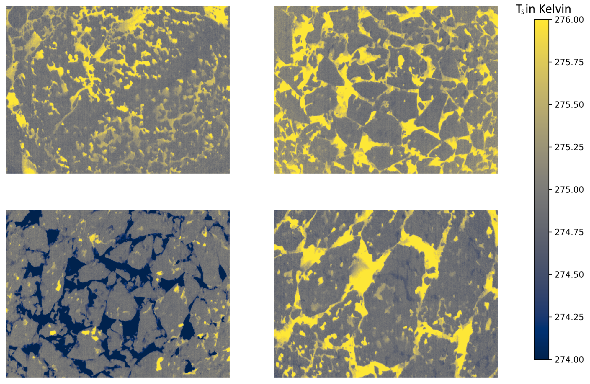
This article focuses on thermal infrared (TIR) imagery instead (Figure 2).15 TIR measures the emissivity of thermal radiation at wavelengths around 10μm. TIR can extend the knowledge gained from VIS retrievals by allowing researchers to ask new questions about the thermal properties of melt ponds, such as heat conductivity. Furthermore, TIR can be used in the absence of daylight. To date, only low-resolution TIR satellite imagery is available. Therefore, TIR data is gathered by helicopter. The gathered data is then analysed and separated according to surface types. 

Figure 2: Ice floes with melt ponds depicted in thermal infrared (TIR) imagery. In some cases, sea ice has a lower temperature than the surrounding ocean (upper left and right, and lower right), in others the opposite is true (lower left). Yellow corresponds to warm, while blue to cold temperatures, as shown on the scale on the right (surface temperatures TS in Kelvin). Images are pseudo-coloured for visibility reasons. Location: Fram Strait region. Date: July 18, 2022 (Source: as above).

How TIR Segmentation Works

Semantic segmentation is an image analysis technique used to classify each pixel into a predefined category. 

In VIS, segementation is often achieved through traditional image processing techniques such as thresholding,16 in which a pixel value threshold is set to differentiate areas of different surface types. Other techniques have used edge detection methods to partition objects from images.17

For TIR imagery, spatially and temporally varying temperatures place special demands on the segmentation algorithm used. Due to its salinity, ocean water has a freezing temperature of -1.8 degrees Celsius. This means that sea ice can be warmer or colder than the surrounding ocean in summer (Figure 2). Simple thresholding approaches are not useful because the surface types can not be distinguished by their pixel value. Furthermore, object boundaries in TIR are challenged by smooth temperature transitions or no transitions at all (Figure 3).

TIR segmentation thus requires a more general method that can consider multiple features such as shape and size simultaneously. Deep learning-based approaches have the potential to help with TIR segmentation because they can learn complex patterns from data. So far, only a few studies have applied deep learning to melt pond segmentation.18
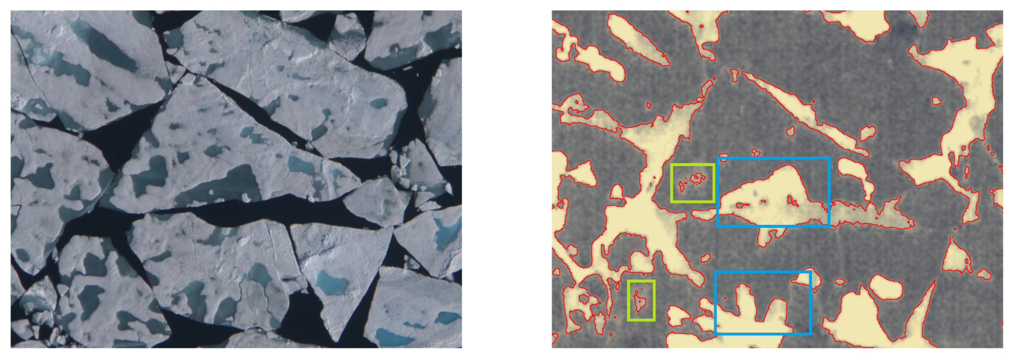
Figure 3: Edge-based segmentation has difficulty distinguishing submerged ice from ocean (blue rectangles) and cannot detect melt ponds with small temperature changes (green rectangles). For this example, a Scharr filter was used (red outlines, Hanno Scharr: Optimale Operatoren in der digitalen Bildverarbeitung. PhD thesis 2000, unpublished manuscript). Yellow corresponds to warm temperatures, while gray/blue to cold ones (right image). Location: Fram Strait region. Date: July 18, 2022 (Source: as above).

Feature Extraction with Convolutional Neural Networks

Deep learning involves a variety of architectures that mimic the neural network structure of the human brain.19 In particular, convolutional neural networks (CNN) are designed for feature extraction from image data.20 They excel at automatically learning patterns at different levels of abstraction, e.g., they can capture local features and spatial context simultaneously. For example, a CNN can recognise that a circular shape alone does not necessarily indicate a melt pond, but must also be embedded in sea ice to differentiate it from an ice floe. This is done using so-called convolutional layers, which apply mathematical operations in the form of filters to the image dimensions.

Semantic Segmentation with U-net

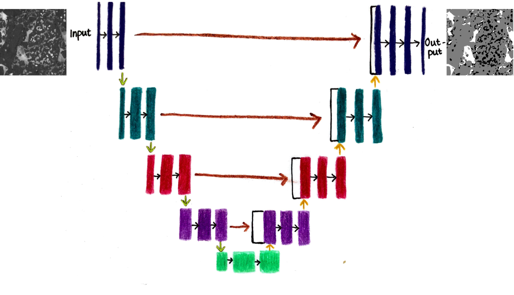
To be suitable for the task of segmentation, a convolutional neural network (CNN) needs to be embedded in a more complex architecture that is able to map the learned features back to the pixel space. A famous architecture in this respect is U-net.21 U-net combines a CNN as a downscaling path with a decoder that upscales the feature representation and outputs a segmentation map (Figure 4).

U-net has achieved significant results in a variety of fields, including satellite image analysis,22 and is one of the most widely used architectures in remote sensing.23 U-net was therefore the model of choice for my work.

Figure 4: Basic U-net architecture. The original image is reduced to a feature representation, which is then upsampled to the original image size. The output is a mask where each pixel is labeled according to category. Ideally, the network is trained by seeing a large number of image-mask pairs, after which it can infer the segmentation map from unseen samples.

Training of Deep Learning Models

To be able to perform well on unseen images, deep learning models must be trained on a large amount of labeled data, typically consisting of thousands or millions of images. This training data needs to be representative, ideally including observations under a variety of conditions. This is challenging for the task of melt pond segmentation, where image acquisition is limited and manual labeling is time-consuming. In practice, several hours of work are required to annotate a single image. 

U-net has been shown to perform well even with relatively few training images.24 In addition, performance results can be improved using techniques such as augmentation and pre-training. Augmentation means transforming existing training data in advance to increase the variation of the dataset.25 This can be done by operations such as flipping or rotating input images. Pre-trained models that have already learned general features from a much larger dataset can be adapted to the task as well.26

Experiments and Results

To test U-net’s usefulness for detecting melt ponds using TIR, I labeled ten TIR images taken during a helicopter flight during the PS131 ATWAICE 2022 campaign.27 I used a U-net pre-trained on ImageNet, one of the largest datasets available for machine learning.28 I optimised some of the configurable hyperparameters, such as the loss function, the patch size and the pre-training strategy, over several training setups and tested different augmentation techniques.29

The results are shown in Figure 5. While some images can be predicted relatively well, this is not the case everywhere. In particular, images taken on a different flight than the training data were segmented incorrectly. 
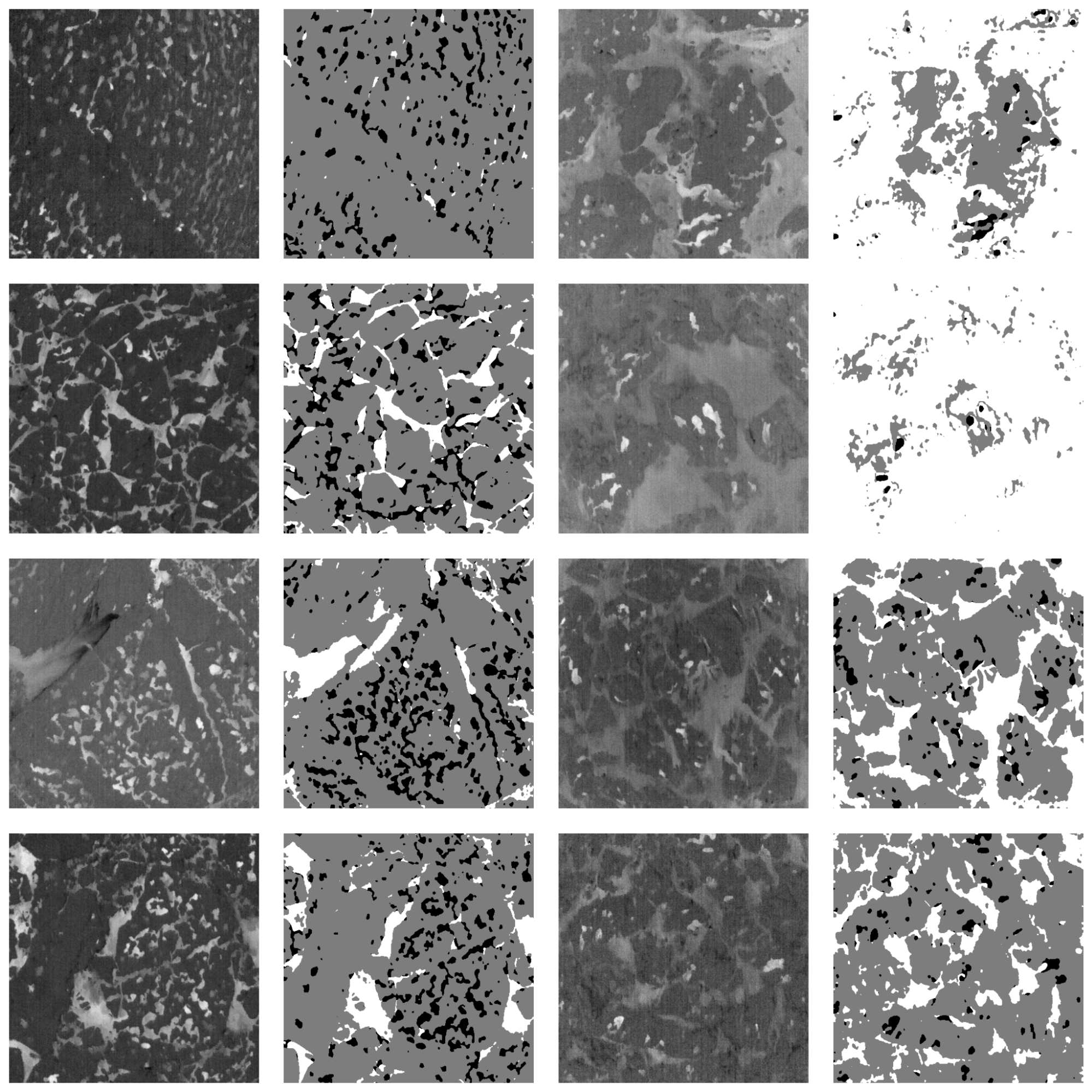
Figure 5: Inference examples on unseen images after training with 10 images. Columns from left to right: sample images from the same flight as the training images; U-net predictions; sample images from a different flight; and U-net predictions. Prediction legend: black - melt pond; gray - sea ice; and white - ocean. To improve the model results, more training is needed, ideally with images from different flights, seasons and areas.

Conclusion

Achieving accurate segmentation of TIR images would open avenues for better understanding the characteristics of Arctic sea ice during the summer. Deep learning methods can help with the challenging task of TIR segmentation, as shown by its successful predictions in the second column of Figure 5. So far, the generalisability of the model is hampered due to limited training data. The development of an operational method remains an ongoing research area, with a particular need to label more representative training data from different flights and areas.


Footnotes
29

This work is based on my Bachelor thesis in the fulfillment of the Cognitive Science degree at the University of Osnabrück in cooperation with the Remote Sensing of Polar Regions research group at the University of Bremen. At the time of publication, the data used in the experiments have not been published. In this regard, I would like to thank my supervisors Dr. Ulf Krumnack and Dr. Gunnar Spreen for their support. I am grateful to Lena Buth from the Alfred Wegener Institute for kindly providing the VIS images used in this article. A special thanks goes to the whole Polar Remote Sensing group for welcoming me into their group and giving me insight into a fascinating field of research.

Mika Rantanen et al.: The Arctic has warmed nearly four times faster than the globe since 1979. In: Communications Earth Environment. Volume 3, 2022, p. 168. 

Dirk Notz, Julienne Stroeve: The trajectory towards a seasonally ice-free Arctic Ocean. In: Current Climate Change Reports. Volume 4, 2018, pp. 407–416.

Jennifer A. Francis, Stephen J. Vavrus: Evidence for a wavier jet stream in response to rapid Arctic warming. In: Environmental Research Letters. Volume 10, No. 1, 2015, p. 014005.

Grete K. Hovelsrud et al.: Arctic societies, cultures, and peoples in a changing cryosphere. In: Ambio. Volume 40, 2011, pp. 100–110; Victor M. Eguíluz et al.: A quantitative assessment of Arctic shipping in 2010–2014. In: Scientific reports. Volume 6, No.1, 2016, pp. 1–6.

 H. Eicken et al.: Tracer studies of pathways and rates of meltwater transport through Arctic summer sea ice. In: Journal of Geophysical Research: Oceans. 2002.; D. K. Perovich, W. B. Tucker III, K. A. Ligett: Aerial observations of the evolution of ice surface conditions during summer. In: Journal of Geophysical Research: Oceans. 2002.

Florence Fetterer, Norbert Untersteiner: Observations of melt ponds on Arctic sea ice. In: Journal of Geophysical Research: Oceans. 1998; Thomas C. Grenfell, Gary A. Maykut: The Optical Properties of Ice and Snow in the Arctic Basin. In: Journal of Glaciology. 2017; Thomas C. Grenfell, Donald K. Perovich: Spectral albedos of sea ice and incident solar irradiance in the southern Beaufort Sea. In: Journal of Geophysical Research: Oceans. 1984, pp. 3573–3580; Grenfell, Perovich: Seasonal and spatial evolution of albedo in a snow-ice-land-ocean environment. In: Journal of Geophysical Research: Oceans. 2004; Marcel Nicolaus et al.: Seasonality of spectral albedo and transmittance as observed in the Arctic Transpolar Drift in 2007. In: Journal of Geophysical Research: Oceans. 2010. 

Chris Polashenski, Donald Perovich, Zoe Courville: The mechanisms of sea ice melt pond formation and evolution. In: Journal of Geophysical Research: Oceans. 2012.

 H. Eicken et al.: Hydraulic controls of summer Arctic pack ice albedo. In: Journal of Geophysical Research: Oceans. 2004.

Daniela Flocco, Daniel L. Feltham, Adrian K. Turner: Incorporation of a physically based melt pond scheme into the sea ice component of a climate model. In: Journal of Geophysical Research: Oceans. 2010; Daniela Flocco et al.: Impact of melt ponds on Arctic sea ice simulations from 1990 to 2007. In: Journal of Geophysical Research: Oceans. 2012; Elizabeth C. Hunke, David A. Hebert, Olivier Lecomte: Level-ice melt ponds in the Los Alamos sea ice model, CICE. In: Ocean Modelling. Volume 71, 2013, pp. 26–42; Chris Polashenski, Donald Perovich, Zoe Courville: The mechanisms of sea ice melt pond formation and evolution. In: Journal of Geophysical Research: Oceans. 2012; Schröder, David et al.: September Arctic sea-ice minimum predicted by spring melt-pond fraction. In: Nature Climate Change. Volume 4, No. 5, 2014, pp. 353–357.

 N. C. Wright, C. M. Polashenski: Open-source algorithm for detecting sea ice surface features in high-resolution optical imagery. In: The Cryosphere. Volume 12, No. 4, 2018, pp. 1307–1329.

e. g., Hannah Niehaus et al.: Sea Ice Melt Pond Fraction Derived From Sentinel-2 Data: Along the MOSAiC Drift and Arctic-Wide. In: Geophysical Research Letters. Volume 50, No. 5, 2023;  L. Istomina et al.: Melt pond fraction and spectral sea ice albedo retrieval from MERIS data – Part 1: Validation against in situ, aerial, and ship cruise data. In: The Cryosphere. Volume 9, No. 4, 2015, pp. 1551–1566. 

e. g., Peng Lu et al.: Sea ice surface features in Arctic summer 2008: Aerial observations. In: Remote Sensing of Environment. Volume 114, No. 4, 2010, pp. 693–699; D. K. Perovich, W. B. Tucker III, K. A. Ligett: Aerial observations of the evolution of ice surface conditions during summer. In: Journal of Geophysical Research: Oceans. 2002; Hannah Niehaus et al.: Sea Ice Melt Pond Fraction Derived From Sentinel-2 Data: Along the MOSAiC Drift and Arctic-Wide. In: Geophysical Research Letters. Volume 50, No. 5, 2023; Nicholas C. Wright, Chris M. Polashenski: How Machine Learning and High-Resolution Imagery Can Improve Melt Pond Retrieval From MODIS Over Current Spectral Unmixing Techniques. In: Journal of Geophysical Research: Oceans. 2020.

Donald K. Perovich et al.: The optical properties of sea ice. In: Monograph. Volume 96, No. 1, 1996.

Linda Thielke et al.: Sea ice surface temperatures from helicopter-borne thermal infrared imaging during the MOSAiC expedition. In: Scientific Data. Volume 9, No. 1, 1996, p. 364.

Peng Lu et al.: Sea ice surface features in Arctic summer 2008: Aerial observations. In: Remote Sensing of Environment. Volume 114, No. 4, 2010, pp. 693–699; D. K. Perovich, W. B. Tucker III, K. A. Ligett: Aerial observations of the evolution of ice surface conditions during summer. In: Journal of Geophysical Research: Oceans. 2002; Mark A. Tschudi, J. A. Curry, J. A. Maslanik: Airborne observations of summertime surface features and their effect on surface albedo during FIRE/SHEBA. In: Journal of Geophysical Research: Atmospheres. Volume 106, No. 14, 2001, pp. 15335–15344; Thomas Krumpen et al.: HELIOS, a nadir-looking sea ice monitoring camera. In: Cold Regions Science and Technology. Volume 65, No. 3, 2011, pp. 308–313; Jun Inoue, Judith A Curry, James A Maslanik: Application of Aerosondes to melt-pond observations over Arctic sea ice. In: Journal of Atmospheric and Oceanic technology. Volume 25, No. 2, 2008, pp. 327–334; W. Huang et al.: Melt pond distribution and geometry in high Arctic sea ice derived from aerial investigations. In: Annals of Glaciology. Volume 57, 2016.

Xin Miao et al.: Object-based detection of Arctic sea ice and melt ponds using high spatial resolution aerial photographs. In: Cold Regions Science and Technology. Volume 119, 2015, pp. 211–222. doi: https://doi .org/10 .1016/j.coldregions.2015.06.014; N. C. Wright, C. M. Polashenski: Open-source algorithm for detecting sea ice surface features in high-resolution optical imagery. In: The Cryosphere. Volume 12, No. 4, 2018, pp. 1307–1329.

Sanggyun Lee et al.: Machine learning approaches to retrieve pan-Arctic melt visible satellite imagery. In: Remote Sensing of Environment. Volume 247, 2020, p. 111919; Nabil Panchi, Ekaterina Kim, Anirban Bhattacharyya: Supplementing Remote Sensing of Ice: Deep Learning-Based Image Segmentation System for Automatic Detection and Localization of Sea-ice Formations From Close-Range Optical Images In: IEEE Sensors Journal. Volume 21, No. 16, 2021, pp. 18004–18019; Ivan Sudakow et al.: MeltPondNet: A Swin Transformer U-Net for Detection of Melt Ponds on Arctic Sea Ice. In: IEEE Journal of Selected Topics in Applied Earth Observations and Remote Sensing. Volume 15, 2022, pp. 8776–8784.

Yann LeCun, Yoshua Bengio, Geoffrey Hinton: Deep learning. In: Nature. Volume 521.7553, 2015, pp. 436–444.

Keiron O’Shea, Ryan Nash: An Introduction to Convolutional Neural Networks. In: arXiv. arXiv:1511.08458, 2015. 

Olaf Ronneberger, Philipp Fischer, Thomas Brox: U-Net: Convolutional Networks for Biomedical Image Segmentation. In: arXiv. arXiv: 1505.04597, 2015.

Benjamin, MatvL, midaha, PGibson, RMcKinlay, Wendy Kan: (2016). Dstl Satellite Imagery Feature Detection. Kaggle. 2016; Vladimir Iglovikov, Sergey Mushinskiy, Vladimir Osin: Satellite Imagery Feature Detection using Deep Convolutional Neural Network: A Kaggle Competition. In: arXiv. arXiv: 1706.06169, 2017.

Thorsten Hoeser, Felix Bachofer, Claudia Kuenzer: Object Detection and Image Segmentation with Deep Learning on Earth Observation Data: A Review—Part II: Applications. In: Remote Sensing. Volume 12, No. 18, 2020.

Olaf Ronneberger, Philipp Fischer, Thomas Brox: U-Net: Convolutional Networks for Biomedical Image Segmentation. In: arXiv. arXiv: 1505.04597, 2015.

Connor Shorten, Taghi M Khoshgoftaar: A survey on image data augmentation for deep learning. In: Journal of big data. Volume 6, No. 1, 2019, pp. 1–48.

Karl Weiss, Taghi M. Khoshgoftaar, DingDing Wang: A survey of transfer learning. In: Journal of Big data. Volume 3, No. 1, 2016, pp. 1–40; Ling Shao, Fan Zhu, Xuelong Li: Transfer learning for visual categorization: A survey. In: IEEE transactions on neural networks and learning systems. Volume 26, No. 5, 2014, pp. 1019–1034.

For more information on the infrared camera see Linda Thielke et al.: Sea ice surface temperatures from helicopter-borne thermal infrared imaging during the MOSAiC expedition. In: Scientific Data. Volume 9, No. 1, 2022, p. 364; For the cruise report see Thorsten Kanzow: The Expedition PS131 of the Research Vessel POLARSTERN to the Fram Strait in 2022. Ed. by Horst Bornemann and Susan Amir Sawadkuhi. Bremerhaven 2023. 

Jia Deng, Wei Dong, R. Socher, Li-Jia Li, Kai Li, Li Fei-Fei: ImageNet: A large-scale hierarchical image database. In: CVPR 2009 – IEEE Conference on Computer Vision and Pattern Recognition, 2009. Juni 2009, pp. 248–255.

I tested methods like flipping and rotating the images to simulate changes in the flight orientation. I also tested to sharpen and blur the images to increase the variety of the dataset. In my experiments, only sharpening and blurring resulted in performance improvement. Code and more details about our experimental setup are available in our GitHub repository

Tags

Related Articles

Jet streams compensate for temperature differences between the equator and the poles and are considered to be relatively stable and reliable winds that can sustain themselves for several days. They are the strongest winds on earth with speeds up to 500 km/h and circulate far above the earth's surface at a height of 9-16 km.

Feedback mechanisms are the processes that amplify or diminish the effects of environmental changes, leading to further shifts in the climate system. An important example is the ice-albedo feedback, where the melting of sea ice exposes darker ocean surfaces that absorb more sunlight and accelerate further ice melt.

A sensor is an instrument on a satellite or helicopter that collects data from the Earth. Different types of sensors are used to detect specific wavelengths of electromagnetic radiation and allow researchers to analyse different aspects of the Earth's surface. For example, optical sensors can be used to distinguish between different types of land cover, such as forests, agricultural land, or urban areas, while thermal sensors can detect changes in temperature.

Emissivity is a physical property that characterises the efficiency with which a surface emits thermal energy. The data is compared to the emissivity of a perfectly black body at the same temperature.

Thermal conductivity is the ability of a melt pond to transfer heat. A higher conductivity means that heat can transfer more efficiently through the melt pond.

Thresholding is an image processing technique that converts an image into a binary form by selecting an appropriate threshold value. Pixels in the image are categorised as either belonging to the foreground or background based on their intensity values in relation to the chosen threshold. By setting multiple thresholds, it is possible to extract multiple classes.

Edge detection is an image processing technique used to identify object boundaries within an image. It often uses large variations in pixel intensities to distinguish entities. During segmentation, the identified objects are classified into different categories, for example, based on their colour.

Segmentation algorithm here refers to the method used to categorise the image pixels.

Deep learning is a category of machine learning methods based on particularly deep artificial neural networks. Deep is defined as any artificial neural network that has at least three layers. While such models were little used at the end of the 20th century due to limited computing capacities, this definition applies to almost every artificial neural network today.

Convolutional neural networks (CNN) form filters to recognise patterns, such as objects in images. Each filter detects the presence of characteristic patterns in the input.

In U-net, the downscaling path refers to the network part that condenses the input image into a simplified representation, which enables the model to extract key patterns. The decoder in U-net works in the opposite direction of the downscaling path. It takes the simplified representation from the downscaling path and reconstructs it back into a more detailed form, aiming to produce an output that closely resembles the original input. A segmentation map is the final output of the image segmentation process. It provides a visual representation where different parts of the input image are categorized into classes.

AI systems are trained for their tasks with data. There are two fundamentally different training methods: supervised and unsupervised learning. In supervised learning, labeled data consisting of pairs of input (e.g., an image) and the desired output of the AI (e.g., the description of the image) is input. This allows the AI to generate image descriptions with feedback. In unsupervised learning, the AI only has a large amount of data (e.g., very many images) at its disposal, but no further information about each individual image. In this second method, the AI must learn to group similar images together.

PS131 ATWAICE was an Arctic expedition conducted on the research vessel Polarstern in the summer of 2022. Scientists from different disciplines joined together to investigate diverse phenomena from ice melt processes and climate change effects on flora and fauna, to glacier melt.

Loss functions are mathematical functions used in machine learning to estimate how well a model is performing. They measure how far the model's predictions are from the actual answers during training. This helps the model to learn and improve its predictions over time.

Patch size refers to the size of the images used for training. For some runs, I divided the images into smaller parts, which increases the training dataset size. However, with a smaller patch size, the spatial context that the model sees decreases. This can make it more difficult for the model to accurately infer the correct class. I found that training on the entire images (with 480x480 pixel size) gave the best results.

There are several ways to use pre-training. Fine-tuning involves continuing to train a pre-trained model on the target task. Freezing refers to a method where the weights of certain layers of a pre-trained model are retained and only the remaining part of the model is trained on the new data set. In my experiment for this article, the best results were obtained with fine-tuning.

Discussions
0 comments
There are new comments!
Te.ma is in archive mode and new comments are disabled.

No comments yet

te.ma does not use cookies. To comply with the General Data Protection Regulation (GDPR), we however have to inform you that embedded media (e.g. from YouTube) may use cookies. You can find more information in our privacy policy.